What is Reinforcement Learning?
Reinforcement Learning (RL) is a subfield of machine learning that focuses on training intelligent agents to make sequential decisions in dynamic environments.
It draws inspiration from how humans and animals learn through trial and error and adapt their behavior to maximize rewards or achieve specific goals.
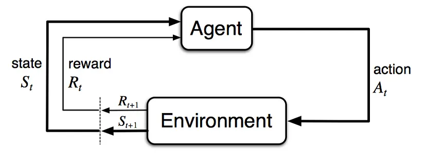
In reinforcement learning, an agent interacts with an environment and learns to take actions to maximize cumulative rewards over time. The environment typically presents the agent with states, which represent different situations or configurations, and the agent's actions can influence the state transitions and the rewards received.
Reinforcement Learning is a fascinating field of AI, and what made us want to explore it further in detail is its similarity to how biological intelligence learns: exploration of the environment, accumulation of knowledge, use of the learning to handle unseen situations.
In order to deepen our comprehension of the mechanisms behind such topic we decided to implement the POLICY GRADIENT ALGORITHM REINFORCE as our project.
We will try to achieve good result with our models on some OpenAI's environments, suchs as the cart-pole and the lunar-lander, and explore related algorithms and ways to further improve Policy Gradient Descent, such as Proximal Policy Optimization.
POLICY GRADIENT
OVERTURE
Markov Decision Processes
Before starting implementing Policy Gradient Descent we take a brief introduction to its background.
"All goals can be described by the maximization of the expected cumulative reward." - The Reward Hypothesis
In order to understand why RL works, we introduce Markov Decision Processes (MDPs), as they provide the formal framework for studying and solving RL problems.
At its core, RL aims to enable an agent to learn how to make sequential decisions in an uncertain environment to maximize cumulative rewards. MDPs provide a systematic way to represent and model such decision-making problems.
An MDP encapsulates the set of possible states, actions, transition probabilities, and reward functions, forming a comprehensive representation of the environment's dynamics and the agent's interactions with it.
A (Discounted) Markov Decision Process (MDP) is a tuple (S,A,R,p,γ), such that

In simple words, an MDP defines the probability of transitioning into a new state, getting some reward given the current state and the execution of an action.
Policy
The dynamics of the environment p are outside the control of the agent. However it can follow a policy ${\pi(a|s)}$, to decide wich action to take given the state.
Following a policy the agent generates a trajectory, a sequence of states, actions and rewards: $S_0, A_0, R_1, S_1, A_1, R_2,...$
Policy: A policy is defined as the probability distribution of actions given a state

The primary objective of RL is to learn an optimal policy that maximizes the expected cumulative reward over time. RL algorithms iteratively update and improve the policy based on feedback from the environment, such as rewards obtained through interactions. By refining the policy, the agent learns to make better decisions and adapt its behavior to achieve its goals.
In our project we will model a neural network to learn the optimal policy for a specific environment. Hence, in this case, the parameters that parametrize the policy will be the parameters of our Neural Network.
In order to improve the parameters and maximize the expected reward we will require the use of policy gradient (descent)!
Policy Gradient Descent
In order to comprehend and code from scratch Policy Gradient we need to understand the math behind it!
We denote a parametrized policy as $$ J(\theta) = \mathbb{E}_{\pi}[r(t)]$$
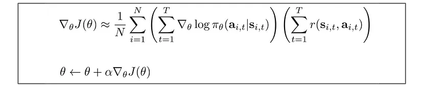
If we find the parameters $\theta \star$ that maximize $J$, the task is solved. The standard approach is to use Gradient Ascent, where the update rule of the parameters is: $$ \theta_{t+1} = \theta_t + \alpha \nabla J (\theta_t)$$ very similar to the update step rule for the parameters of neural networks we have seen during the course, except that there we had to minimize a loss!
To express our objective mathematically we have: The expected rewards equal the sum of the probability of a trajectory × corresponding rewards:
 (where u is the action)
And so we need to maximize them:
 (*)
(*)
In order to optimize we introduce a common trick in Reinforcement Learning:

replacing $f(x)$ with $\pi$: $$ \pi_\theta (\tau)\nabla_\theta log\pi_\theta(\tau) = \nabla_\theta \pi_\theta(\tau)$$
For continuous space the expectation can be expressed as: $$ \mathbb{E}_{X\sim p(x)}[f(x)] = \int p(x)\ f(x)\ dx $$
Now we go back to the maximization of our expectation (*):

as the probability of each step of the trajectory $\tau$ is considered in the expectation (which is probability of the trajectories over the policy parameters), and the reward is the same in both expressions.
We then rewrite our objective function as: $$ J(\theta) = \mathbb{E}_{\tau\sim \pi_\theta(\tau)}[r(\tau)] = \int \pi_\theta (\tau) r(\tau)d\tau$$ And the POLICY GRADIENT becomes:
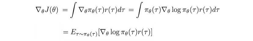
since we use the log-derivative trick and consider the continuous expectation as integral, and back.
The partial derivative of $log \ \pi(\tau)$, which is the log of the policy probabilities over the trajectory $\tau$ is derived in 3 steps:
- I $$ \pi_\theta(\tau)=\pi_\theta(s_1,a_1,...,s_T,a_T)=p(s_1)\prod_{t=1}^T\pi_\theta(a_t|s_t)p(s_{t+1}|s_t,a_t) $$
where we interpret $\pi$ as the policy (prob of taking that action given state) and $p$ as the actual probability of the agent to reach the next state given actual state and action (e.g. the environment may present nuances such as wind, or disturbing forces), so the agent on its trajectory may depend on a probability p to reach next state.
- II
Taking the log lead to: $$ log\pi_\theta(\tau)=log\ p(s_1)+\sum_{t=1}^T log\pi_\theta(a_t|s_t)+log\ p(s_{t+1}|s_t,a_t) $$
- III
Taking the derivative, we see the first and last term does not depend on $\theta$, so the POLICY GRADIENT becomes:
The policy gradient algorithm offers a unique perspective, focusing on directly optimizing the policy, which will provide valuable insights into the decision-making process of intelligent agents!
Altough the main reason why we have chosen this algorithm is because it can directly work on the parameters of a neural network (policy) in a continuous way, the pros of this algorithm are the capability to handle stochastic policies, has converges guarantees, gradient estimation, and model-free learning (does not require explicit knowledge or assumptions about the underlying dynamics of the environment). All of this contribute to its effectivness in a wide range of real-world applications.
REINFORCE ALGORITHM
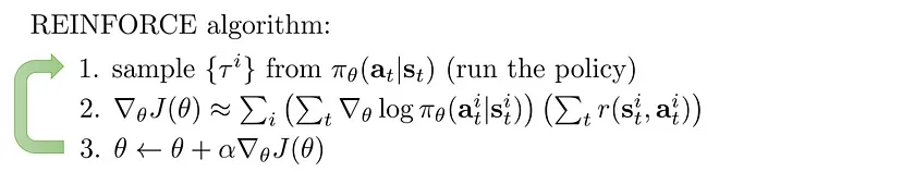
To implement gradient ascent we made use of the REINFORCE Algorithm.
The REINFORCE algorithm is a popular policy gradient method in reinforcement learning that aims to learn an optimal policy directly through gradient ascent. It uses the concept of Monte Carlo sampling to estimate gradients and update the policy parameters iteratively.
The REINFORCE algorithm belongs to the class of on-policy methods because it uses the current policy to collect data and improve the policy iteratively. It directly optimizes the policy parameters using gradient ascent, without explicitly estimating value functions.
Its steps are: Initialize Policy, Collect Trajectories, Compute Return (sum of discounted future rewards), Estimate Policy Gradient, Update Policy, repeat 2-5.
As we can see it is the straighforward iterating use of the policy gradient update.
Our Implementation
We made the choice to make no use of Deep Learning libraries, during the course in fact we have seen how to code a neural network up, and we started from there to implement our agent; this would come at cost of a worsen efficency and sometimes diminished learning, but with a much greater insight and comprehension of the mechanisms that lies behind such intricate topic.
NeuralNetwork.py contains the model for our agent. We won't go through the neural network code as we have seen it during classes and labs, we only made some improvements preparatory to our purposes.
What is worth mentioning is:
- the addition of a Softmax output layer, (function at line 365);
- the implementation of ADAM (Adaptive Moment Estimation) optimizer; briefly it combines the benefits of both adaptive learning rate methods, and momentum-based methods, to achieve efficient and effective optimization. (line 277) -> Actually ADAMw (weight decay)
- We worked on the backpropagation code that gave us some issues.
- Added a new weight initialization: Glorot Init. (line 108)
- We later explore the Reinforcement Learning code used.
Reinforce Gradient
The hardest challenge we went through in our project was the coding of the REINFORCE Algorithm and in particular the coding of the REINFORCE Gradient.
As the ouput layer of our neural network is a Softmax layer, needed to output a distribution over the possible action space, we needed to find the gradient of the REINFORCE loss over the softmax layer.
The loss function in the case of a softmax output is typically the cross-entropy loss, which measures the difference between the predicted probabilities (softmax output) and the true labels.
The cross-entropy loss for a single training example with $K$ classes can be define as: $$ \mathcal{L} = - \sum_{k=1}^K y_k log \hat{y}_k $$
where $y_k$ is the true label (one-hot encoded vector) and $\hat{y}_k$ is the predicted probability for class $k$ (softmax output).
During the REINFORCE algorithm, the loss function can be modified to incorporate the rewards or penalties associated with each action taken by the agent. One common approach is to use the reinforce loss function, which is defined as: $$ \mathcal{L} = - \sum_{t=1}^T log \ \pi(a_t|s_t)R_t $$
where $\pi$ is the policy, $R_t$ is the cumulative reward from time step $t$ to the end of the episode, and $T$ is the total number of time steps in the episode.
We have no label as indeed the reinforcement learning setup doesn't provide for it, however we'll see that the loss depends strictly and solely on the action taken.
NOTE that in the REINFORCE algorithm, the objective is to maximize the expected cumulative reward. However, most optimization algorithms, including gradient descent, usually found in neural networks code, are designed to minimize a loss or cost function. Therefore, to align the objective of maximizing the expected reward with the minimization framework of gradient descent, a negative sign is typically introduced.
By multiplying the REINFORCE loss by -1, the objective becomes minimizing the negative of the expected cumulative reward, which is equivalent to maximizing the expected cumulative reward. This allows the REINFORCE algorithm to be formulated as a minimization problem that can be solved using gradient-based optimization techniques like gradient descent.
- It is also important to note the fact that a specific choice of an action affects both present and future rewards. Future rewards can be discounted by a factor $\gamma$ (discounted rewards), indicating the fact that long in the future rewards depend less on the present action -> ($R_T$ is the cumulative reward from the actual step to the end of the trajectory).
From where does this loss function come from?
- We start from the definition of the policy gradient provided earlier in our definition of expected value of total reward:
this slightly differs from the expression provided earlier for the fact that this is the expectation itself, not the approximation using a batch of trajectories, hence this is a proper equation, expressing the policy gradient theorem.
- We can rewrite the summation inside the expectation as $ \nabla_\theta J(\theta) = \mathbb{E}_{\tau \sim \pi} [\sum_{t=0}^T \nabla_\theta log \pi(a_t|s_t) \cdot R(\tau)] $,
where $R(\tau)$ represents the total reward obtained in the trajectory $\tau$.
In the REINFORCE algorithm, we estimate this gradient using Monte Carlo sampling, and we approximate the expectation by averaging over multiple sampled trajectories.
Looking at the REINFORCE Loss definition, the gradient used to update the policy parameters in the REINFORCE algorithm is indeed $\nabla_{\theta} \mathcal{L} = - \sum_{t=0}^T \nabla_\theta log \pi(a_t|s_t) \cdot R(\tau)$.
NOTE that the REINFORCE loss is negative leading to a negative summation expressed above, however we need an expectation (which is positive): we already know how when maximizing the expected rewards over the trajectories, we can minimize the negative of this expectation to use Neural Networks' gradient descent, so the loss we use in the context of our Neural Network Model instead of maximizing $\nabla_{\theta} \mathcal{L}$ aims to minimize $- \nabla_{\theta} \mathcal{L} = \sum_{t=0}^T \nabla_\theta log \pi(a_t|s_t) \cdot R(\tau)$.
The gradient of the log probabilities is indeed utilized as a way to find the gradient of the REINFORCE loss and ultimately update the policy parameters in the REINFORCE algorithm!
Now we need to utilize this loss in our backpropagation: we need to know how it varies with respect to the softmax output layer.
To compute the gradient of the REINFORCE loss with respect to the softmax output, we used the chain rule of differantion and the following formula:
$$ \frac{\partial\mathcal{L}}{\partial z_k} = \sum_{t=1}^T \frac{\partial\mathcal{L}}{\partial log\ \pi(a_t|s_t)} \frac{\partial log\ \pi(a_t|s_t)}{\partial z_k} $$
where $z_k$ is the output of the last layer for class $k$, $\mathcal{L}$ is the REINFORCE loss function, $\pi(a_t|s_t)$ is the (Policy) probability of taking action $a_t$ given state $s_t$, and $T$ is the total number of time steps in the episode.
First Term:
The first term in the formula represents the gradient of the REINFORCE loss with respect to the logarithm of the action probabilities. This term can be computed using the following formula: $$ \frac{\partial\mathcal{L}}{\partial log\ \pi(a_t|s_t)} = R_T \cdot \mathbb{I}(a_t = k) $$
where $R_t$ is the cumulative reward from time step $t$ to the end of the episode, and $\mathbb{I}(a_t = k)$ is an indicator function that equals 1 if action $a_t$ is equal to class $k$ and 0 otherwise.
DERIVATION:
We now derive the expression for $ \frac{\partial\mathcal{L}}{\partial log\ \pi(a_t|s_t)}$.
Knowing that we can use the REINFORCE Loss to estimate the gradient of the policy parameters we express the loss as an expectation by considering the probability distribution over trajectories $\tau$ generated by following the policy $\pi$:
$$ \mathcal{L} = \mathbb{E}_{\tau \sim \pi} [\sum_{t=0}^T log\pi(a_t|s_t) \cdot R(\tau)] $$
we can rewrite the REINORCE Loss as follows: $ \mathcal{L} = \mathbb{E}_{\tau \sim \pi} [\sum_{t=0}^T (log\pi(a_t|s_t) \cdot R(\tau)) \cdot 1] $, introducing an indicator function by multiplying and dividing by $1$.
We can now rewrite the loss as: $ \mathcal{L} = \mathbb{E}_{\tau \sim \pi} [\sum_{t=0}^T (log\pi(a_t|s_t) \cdot R(\tau)) \cdot \mathbb{I}(a_t=\hat a_t)] $, where $\hat{a}_t$ is the action taken at time step $t$, and $\mathbb{I}(\cdot)$ is the indicator function.
Now, we can compute the derivative with respect to $\log \pi(a_t|s_t)$: $$ \frac{\partial\mathcal{L}}{\partial log\ \pi(a_t|s_t)} = \mathbb{E}_{\tau \sim \pi} [\sum_{t=0}^T \frac{\partial}{\partial log \pi(a_t|s_t)} log\pi(a_t|s_t) \cdot R(\tau) \cdot \mathbb{I}(a_t=\hat a_t)] $$
Now, the derivative term simplifies as follows: $ \frac{\partial}{\partial log \pi(a_t|s_t)} log\pi(a_t|s_t) = 1 $
Therefore we have: $$ \frac{\partial\mathcal{L}}{\partial log\ \pi(a_t|s_t)} = \mathbb{E}_{\tau \sim \pi} [\sum_{t=0}^T 1 \cdot R(\tau) \cdot \mathbb{I}(a_t=\hat a_t)] = \mathbb{E}_{\tau \sim \pi} [\sum_{t=0}^T R(\tau) \cdot \mathbb{I}(a_t=\hat a_t)] $$
This equation is indeed equivalent to the one above, in fact the expectation can be estimated with Monte Carlo sampling, as we do in our code; the summation is computed using the whole trajectory, approximating the total gradient with a summation of the gradient computed at each timestep; $R(\tau)$ represents the cumulative reward obtained in the trajectory, above $R_T$ is the reward over the trajectory until the reward horizon T; $\mathbb{I}(\cdot)$ is the same indicator function.
So in other words, to compute the gradient of each time step over a trajectory (each step of our agent), in a Monte Carlo setting, we use the term: $ R_T \cdot \mathbb{I}(a_t = k) $ equivalent to the expression derived above. And we code this inside the gradient calculation used for the backpropagation in the delta function at line 46.
Second Term:
The second term in the formula represents the gradient of the logarithm of the action probabilities with respect to the input of the last layer. This term can be computed using the following formula: $$ \frac{\partial log\ \pi(a_t|s_t)}{\partial z_k} = \hat{y}_k - \mathbb{I}(a_t = k)$$
where $\hat{y}_k$ is the predicted probability for class $k$ (which is equal to the softmax output), and $\mathbb{I}(a_t = k)$ is an indicator function that equals 1 if action $a_t$ is equal to class $k$ and 0 otherwise.
DERIVATION:
This is the derivative of the log of the softmax with respect to the logits. We used a calculation found here;
essentially it is:
$$ \begin{split}
\frac{\partial}{\partial o_{i}} L &= - \sum_{j=i}y_{j} \frac{\partial \log (p_{j})}{\partial o_{i}} - \sum_{j \neq i}y_{j}\frac{\partial \log (p_{j})}{\partial o_{i}}\\
&= - \sum_{j=i}y_{j} \frac{1}{p_{j}}\frac{\partial p_{j}}{\partial o_{i}} - \sum_{j \neq i}y_{j}\frac{1}{p_{j}}\frac{\partial p_{j}}{\partial o_{i}}\\
&= - y_{i} \frac{1}{p_{j}} p_{j}(1-p_{i}) - \sum_{j \neq i}y_{j}\frac{1}{p_{j}}(-p_{j}p_{i})\\
& = - y_{i} (1- p_{i}) - \sum_{j \neq i}y_{j}\frac{1}{p_{j}}(-p_{j}p_{i})\\
&=- y_{i} + \underbrace{y_{i}p_{i} + \sum_{j \neq i}y_{j}p_{i}}_{ \bigstar } \\
&= p_{i}\left(\sum_{j}y_{j} \right) - y_{i} = p_{i} - y_{i}
\end{split} $$
where $p_i = Softmax(o_i)$ and $y_i$ is the one hot encoded vector (so an indicator).
This is clearly equivalent to the second term above, since $p_i = \hat{y}_k $ is the policy probability for class $k$ (softmax output); and $y_i$ is indeed the same indicator function $\mathbb{I}(a_t = k)$.
The Code
The code for the gradient can be found at line 46, it is something like this:
    def delta(z,a,y,discountedReturn,p):

            first = np.zeros_like(a)
            first[np.argmax(y)] = discountedReturn

            second = a
            second[np.argmax(y)] -= 1

            grad = first * second
            return grad
Here we can see the first term $ R_T \cdot \mathbb{I}(a_t = k) $ is computed as an empty array, with reward only on action selected (action k); (this takes account for the indicator)
while we see that the second term $\hat{y}_k - \mathbb{I}(a_t = k)$ is the array containg the softmax predictions, subtracting 1 on the action taken. (this could also have been done subtracting y from second term)
y is the one-hot encoded vector of the actions.
Thoughts and impressions
The lenghty derivations lead us to a very short gradient calculation, yet we believe we might have missed something: as we will see in our implementations, the agents learning sometimes gets stuck in suboptimal behaviours.
After trying out many different weights initializations, we can't be sure whether it depends on the actual gradient, on the reward shaping or on some very complex scenarios, risen from the highly stochastic nature of the problem instances (we believe the last).
What is sure is that our code is no so optimized, and this could help worsen the convergence to an optimal behaviour, leading to high variance trajectories during learning, nonetheless we'll se how just plain gradient descent achieves very good result in few epochs, even on large networks!
Cart Pole!
We now have all we need to start and make our agents learn!
The environment we have chosen to start from is the Cart-Pole, a problem described by Barto, Sutton, and Anderson in “Neuronlike Adaptive Elements That Can Solve Difficult Learning Control Problem”.
A pole is attached by an un-actuated joint to a cart, which moves along a frictionless track. The pendulum is placed upright on the cart and the goal is to balance the pole by applying forces in the left and right direction on the cart.
CartPole is often considered as one of the classic and beginner-friendly RL environments due to its simplicity and intuitive dynamics.
It serves as a good starting point for understanding RL algorithms and concepts.
Details:
Action Space
- 0: Push cart to the left
- 1: Push cart to the right
Observation Space
- The observation is an array with shape 4 with values corresponding to:
- Cart Position,
- Cart Velocity,
- Pole Angle,
- Pole Angular Velocity.
Rewards
Since the goal is to keep the pole upright for as long as possible, a reward of +1 for every step taken, including the termination step, is allotted.
Episod End
The episode ends if any one of the following occurs:
Termination: Pole Angle is greater than ±12°
Termination: Cart Position is greater than ±2.4 (center of the cart reaches the edge of the display)
Truncation: Episode length is greater than 500
Needed libraries are:
- gymnasium or gym (one of the two is fine):
- pip install gym
- pip install gymnasium
- matplotlib: pip install matplotlib
- numpy: pip install numpy
They can all be installed using pip.
# import needed libraries
import gymnasium as gym
from matplotlib import pyplot as plt
# from IPython.display import clear_output
import numpy as np
import random
import NeuralNetwork
We now define some of the functions we need for our agent, we will go through each of them as we define them
Discounted Rewards
Discounted rewards take into account the fact that future rewards are often worth less than immediate rewards. This is based on the idea of time preference or the notion that immediate rewards are typically more valuable than delayed rewards. The discount factor, denoted by gamma (γ), is a value between 0 and 1 that determines the importance of future rewards relative to immediate rewards.
The discounted reward at a particular time step is calculated by summing the rewards obtained from that time step onward, with each reward multiplied by the corresponding discount factor raised to the power of the number of time steps into the future it is received. Mathematically, the discounted reward at time step t is given by: $$ R_t = r_t + \gamma \cdot r_{t+1} + \gamma^2 \cdot r_{t+2} + \gamma^3 \cdot r_{t+3} + ... + \gamma^T \cdot r_{T} $$ where $r_t$ is the reward at time step $t$, $\gamma$ is the discount factor and $T$ is the lenght of the trajectory.
By discounting future rewards, the agent takes into account the potential risks and uncertainties associated with delayed rewards. It encourages the agent to prioritize immediate rewards while still considering the potential long-term benefits of its actions.
Discounted rewards play a crucial role in reinforcement learning algorithms, such as Q-learning and policy gradient methods, as they provide a mechanism for evaluating and comparing different actions and policies based on their expected cumulative rewards over time.
In the cartpole we set $\gamma = 1$ as is important to signal the fact that future rewards depends on all the actions taken up to that point, since there is no negative reward here, $\gamma = 1$ gives more feedback to initial actions, if there was negative reward, then it could have worsen the learning (e.g. a big negative reward risen form a small set of future actions could disturb initial actions that were right, meaning that it would make the probs of that actions to reduce instead of increase (look at the gradient)).
In the lunar lander discounted rewards are more useful, for the above reason.
def discountedRewards(rewards, gamma=1):
    # in this implementation each discounted reward, starting from the last one, is computed by multipling the following discounted rewards (R) by a factor gamma
    # and adding the actual reward.
    R = 0
    return [R:=(R * gamma + rewards [t]) for t in reversed(range(len(rewards))) ][::-1]
def discountedRewards2(rewards, gamma=1):
    #return np.cumsum(rewards[::-1])[::-1]
    return np.cumsum(rewards * (gamma ** np.arange(len(rewards))))
Epsilon-greedy exploration & Epsilon decay
Epsilon-greedy exploration is a strategy used to balance the exploration-exploitation tradeoff.
Exploration refers to the process of trying out different actions to gather information about the environment, while exploitation refers to using the agent's current knowledge to select actions that are expected to yield the highest immediate reward.
The epsilon-greedy strategy involves selecting the best-known action (exploitation) with a probability of 1-epsilon, and selecting a random action (exploration) with a probability of epsilon. In other words, the agent follows the known best action most of the time, but occasionally explores other actions to discover potentially better strategies.
Epsilon decay is the process of gradually reducing the exploration factor (epsilon) over time. Initially, a high value of epsilon encourages more exploration, but as the agent learns more about the environment, it becomes more beneficial to exploit the known best actions. By decaying epsilon over time, the agent gradually shifts its focus from exploration to exploitation.
# Epsilon-greedy exploration
def sampleSoftmax(softmaxOutput, epsilon):
    if random.uniform(0, 1) < epsilon: # esilon probability to act random
        sampledAction = random.randint(0, len(softmaxOutput) - 1) # random action selected
    else:
        rand = np.random.random()  # uniform distribution generator
        cdf = np.cumsum(softmaxOutput)
        sampledAction = np.argmax(cdf > rand) # inverse sampling to sample actions according to the policy distribution
    return sampledAction, np.log(softmaxOutput[sampledAction][0]+1e-8)
Reward shaping
Reward shaping is a technique used in reinforcement learning to modify the reward signal received by an agent to facilitate learning or improve the learning process.
Reward shaping aims to provide additional feedback to the agent during the learning process by creating intermediate or shaped rewards based on the current state and action. These shaped rewards are designed to guide the agent towards desired behaviors or subgoals, helping it to learn more effectively and efficiently.
The shaped rewards act as a bridge between the sparse and delayed original rewards and can help speed up the learning process by providing more informative and timely feedback to the agent.
However, it's important to note that reward shaping should be done carefully. Poorly designed shaped rewards can lead to suboptimal behavior or unintended side effects.
Overall, reward shaping is a valuable technique in reinforcement learning that can accelerate learning by providing additional feedback to the agent during the learning process, leading to more efficient and effective exploration and exploitation of the environment.
In the case of the Cart-Pole reward shaping can be done by limiting the angle to which the reward is assigned.
Usually a reward of +1 is given for every time step, ignoring the pole angle (or pole angular velocity).
By setting a threshold beyond which the agent take negative reward (-1) may help learn the correct behaviour for our agent
def reward_function(state, alpha=1):
    # Compute the angle between the vertical and the pole
    angle = state[2]
    angularVelocity = state[3]

    # Angle threshold
    angle_threshold = 0.418

    # If the angle exceeds the threshold, penalize the agent
    if abs(angle) > angle_threshold * alpha: reward = -1.0
    else: reward = 1.0

    return reward
Baseline
A baseline refers to a value or function that is used to provide a reference point for comparison when estimating the advantage or value of different actions or states.
The purpose of a baseline is to reduce the variance of the estimated advantages or values. By subtracting a baseline from the estimated quantities, the resulting values are centered around zero, which can make learning more efficient.
The choice of a baseline is important because it should satisfy certain properties. Ideally, a good baseline should be unbiased, meaning that its expected value should be equal to the true advantage or value function being estimated. Additionally, a good baseline should have low variance to reduce the noise in the estimates.
A common choice for a baseline is the state-value function (V) or the action-value function (Q) estimated by the agent. These value functions provide an estimate of the expected cumulative reward from a particular state or state-action pair, respectively. By subtracting the value function from the estimated advantage or action-value, the agent can focus on the relative advantage or difference compared to the average or expected value.
In our project we used two neural networks to learn the state-value function V and the action-value Q, however we did not find a particular improvement in performance by our agent.
We also tried exponential moving average, and all the simpler types of baselines, with no behavioral gains.
def moving_average_baseline(rewards, alpha=0.9):
    baseline = 0
    baselines = []
    for r in rewards:
        baseline = alpha * baseline + (1 - alpha) * r
        baselines.append(baseline)
    return np.array(baselines)
def exponential_moving_average2(values, alpha):
    ema = [values[0]]
    for i in range(1, len(values)):
        ema.append(alpha * values[i] + (1 - alpha) * ema[i-1])
    return ema
def exponential_moving_average(prev, actual, alpha=0.8):
    return alpha*actual + (1-alpha) * prev
Imitation Learning
Imitation learning is a technique in machine learning where an agent learns a policy or behavior by imitating demonstrations or examples provided by an expert. The goal is to learn from the expert's behavior and generalize it to make good decisions in similar situations.
The process of imitation learning typically involves two main components: the expert policy and the learning algorithm. The expert policy is a pre-existing policy that demonstrates the desired behavior. It could be a human demonstrator or an expert algorithm. The learning algorithm uses the expert's demonstrations as training data to learn a policy that mimics the expert's behavior.
There are several related techniques and approaches in imitation learning: Behavior Cloning, Inverse Reinforcement Learning, Generative Adversarial Imitation Learning (GAIL), Apprenticeship Learning.
Altough imitation learning techiniques are very vast, we chose not to go too deep into it, it is extremely charming (especially GAIL!), however we had limited resources and chose to wait on it, it will for sure be a future study topic.
Reason of this choice were that starting from scratch we didn't already have optimal working policies, and that we preferred to make our agent learn from zero, using only rewards.
Nothing stopped us however to use behavior cloning on new nets using the agents that learned properly, doing so helped in some cases the convergence.
Learning Process!
- Critic is the net we used for practicing imitation learning
import NeuralNetwork
critic = NeuralNetwork.load('../DeepLearningProject/Networks/800') # THe net that is used to dictate the best actions
- trainAgent is the function used to make agent learn the CartPole, it contains every sperimentation we did in order to achieve good results.
def trainAgent(model,env, ValueNet, QNet, trainNets=False, randomExploration = 0, angleTreshold = 1, learninRate =  0.01, lambda_=0, iterationAmplification = 1, critic=None, print_=True):
    # reset the environment and observe it
    envStates = env.observation_space.shape[0]
    env.action_space.seed()

    observation, info = env.reset()
    observation = observation.reshape(envStates,1)

    learningScore = []
    rewards = []
    trueRewards = []
    probs = []
    actions = []
    states = []
    savedLogProbs = []
    savedProbs = []
    actionIndexes=[]
    actionSingleIndex=[]
    replayBuffer=[]
    game = 1
    # randomExploration: hyperparameter to incentive random exploration (random actions)
    # angleTreshold: hyperparameter that regulates the maximum rewarding angle
    eta=learninRate
    meanReward = 0
    baseline = 0
    maxScore = 0
    interval = min(100, iterationAmplification)
    prev_avg_reward = 0 # baseline
    breakFlag = False
    lastMean=0
    imitate = False
    batch = 0
    advantageList = np.array([])

    # Main loop
    while(True):
        observation = observation.reshape(envStates,1)
        states.append(observation)
        # Policy probabilities
        prob = model.feedForward(np.array(observation))
        # Policy Action selection
        action, lP = sampleSoftmax(prob, randomExploration)

        # Imitation Learning
        if imitate and np.random.random()<0.5:
            criticAction, _ = sampleSoftmax(critic.feedForward(np.array(observation)), 0)
            lP = np.log(prob[criticAction])
            action=criticAction

        # Agent makes the action
        observation, trueReward, terminated, truncated, info = env.step(action)
        # Reward shaping
        reward = reward_function(observation, angleTreshold)
        # One-hot encoded vector
        y = tuple([1 if i==action else 0 for i in range(len(prob))])

        probs.append(prob)
        actions.append(y)
        rewards.append(reward)
        trueRewards.append(trueReward)
        savedLogProbs.append(lP)
        savedProbs.append(prob[action])
        actionIndexes.append(np.array([action]))
        actionSingleIndex.append(action)

        # Episode terminaed
        if terminated or truncated:
            meanReward += sum(trueRewards)
            game += 1
            states.append(observation)
            # baseline = (baseline *(game-1) + sum(rewards)) / game

            # Hyperparameter Annealing:     Slowly modify hyperparameters in order to help the learning
            if not game%interval:
                meanReward /= interval
                if print_: print(f' game: {game}, mean reward: {meanReward}, at eta: {eta}, exp: {randomExploration}, angle: {angleTreshold}, lambda: {lambda_}')
                learningScore.append((game, meanReward))
                if meanReward >= 500: breakFlag=True; break
                if game==iterationAmplification: breakFlag=True; break
                if meanReward>=400: eta = 0.0001; randomExploration = 0.01;  angleTreshold=.5
                elif meanReward>=100: eta = 0.005; randomExploration=0.05; angleTreshold=.8
                elif meanReward<20: randomExploration=0.8; eta=0.01;
                else: eta = 0.001; randomExploration = 0.05; angleTreshold=1
                #if game>1000 and game<2000 and meanReward<22: breakFlag=True
                # if game==200 and meanReward<=22: breakFlag=True
                meanReward = 0
                trueRewards=[]


            # Obtaining the discounted rewards
            dR = discountedRewards(rewards, .9)

            advantage = dR # discounted rewards used as advantageS


            # Training of the State-Value net and of the Action-Value net for a better baseline and advantage
            if trainNets:
                gamma=0.99
                valueStates=[]
                actionvalueStates=[]
                for i in range(len(rewards)):
                            # ValueNet estimates
                            V_next_estimate = ValueNet.feedForward(states[i])
                            Vs = rewards[i] + gamma * V_next_estimate
                            valueStates.append(Vs)
                            # QNet estimates
                            actionValueVector=[QNet.feedForward(np.append(states[i], [action]))[action] for action in range(env.action_space.n)]
                            actionValueVector = [el.tolist() for el in actionValueVector]
                            Q_next_state = QNet.feedForward(np.append(states[i], actionSingleIndex[i]))[actionSingleIndex[i]]
                            actionValueVector[actionSingleIndex[i]] = [rewards[i] + gamma * np.max(Q_next_state)]
                            actionvalueStates.append(np.array(actionValueVector).reshape(-1))

                V_train = [(state,target) for state, target in zip(states, valueStates+[0])]
                Q_train = [(np.append(state,[action]).reshape(-1,1), target.reshape(-1)) for state, action, target in zip(states[:-1], actionSingleIndex, actionvalueStates)]

                ValueNet.SGD(V_train, 20, 64, 0.1)
                QNet.SGD(Q_train, 20, 64, 0.1)

                advantage = [QNet.feedForward(np.append(states[i], actionSingleIndex[i])) - ValueNet.feedForward(states[i]) for i in range(len(rewards))]
                advantage = [el[0] for el in advantage]


            #returns = np.array(dR)
            returns = np.array(advantage)

            # scaling and normalization of the returns in order to reduce their variance and improve learning
            eps = np.finfo(np.float32).eps.item()
            returns = (returns - returns.mean()) / (returns.std() + eps)
            returns = np.array(returns)

            advantageList = np.append(advantageList, returns)

            rewards = []
            batch += 1
            if not batch%32:
                batch = 0

                # apply Policy Gradient Descent
                model.PolicyGradientDescent(states, actions, advantageList, probs, eta=eta, lambda_=lambda_)


                # Proximal Policy Optimization: not used on CartPole


                '''currentProb=[]
                for state in states:
                    prob = model.feedForward(np.array(state))
                    currentProb.append(prob)

                model.ProximalPolicyOptmization(states, actions, advantageList, probs, currentProb, eta=eta, lambda_=lambda_)'''


                # Replay Buffer: Not used on CartPole
                '''
                replayBuffer.append((states, actions, returns, probs, game))
                #replayBuffer.sort(key=lambda x:len(x[1]), reverse=True)
                #replayBuffer.sort(key=lambda x:len(x[1]))
                #replayBuffer = [el for el in replayBuffer if game - el[4]<5 and len(el[1])>90]

                if len(replayBuffer)>1000:
                    replayBuffer.pop(0)

                #if np.random.random()<=0.01:

                indices = random.sample(range(0, len(replayBuffer)), k=min(5, len(replayBuffer)))
                for i in indices:
                    traj = replayBuffer[i]
                    model.PolicyGradientDescent(*traj[:-1], eta=eta, lambda_=lambda_)'''

                advantageList = np.array([])
                probs = []
                actions = []
                rewards = []
                trueRewards=[]
                states = []
                observation, info = env.reset()
            if breakFlag: break


    env.close()
    return learningScore
- useful functions below
def showAgent(model,env, games=10, flag=False):
    observation, info = env.reset()
    envStates = env.observation_space.shape[0]
    observation = observation.reshape(envStates,1)
    rewards = []

    while games:
        observation = observation.reshape(envStates,1)
        prob = model.feedForward(np.array(observation))
        action, _ = sampleSoftmax(prob, 0)
        observation, reward, terminated, truncated, info = env.step(action)
        rewards.append(reward)

        if terminated or truncated:
            if flag: print(sum(rewards))
            rewards = []
            observation, info = env.reset()
            games-=1

    env.close()
def train_V_Q_Nets(model, env, ValueNet, QNet, games=10, epochs=100, gamma=0.95, flag=False):
    observation, info = env.reset()
    envStates = env.observation_space.shape[0]
    observation = observation.reshape(envStates,1)
    rewards = []
    states = []
    actionSingleIndex = []

    while games:
        observation = observation.reshape(envStates,1)
        states.append(observation)
        prob = model.feedForward(np.array(observation))
        action, _ = sampleSoftmax(prob, 0)
        observation, reward, terminated, truncated, info = env.step(action)
        rewards.append(reward)
        actionSingleIndex.append(action)

        if terminated or truncated:
            if flag: print(sum(rewards))

            valueStates=[]
            actionvalueStates=[]
            for i in range(len(rewards)):
                        # ValueNet estimates
                        V_next_estimate = ValueNet.feedForward(states[i])
                        Vs = rewards[i] + gamma * V_next_estimate
                        valueStates.append(Vs)
                        # QNet estimates
                        actionValueVector=[QNet.feedForward(np.append(states[i], [action]))[action] for action in range(env.action_space.n)]
                        actionValueVector = [el.tolist() for el in actionValueVector]
                        Q_next_state = QNet.feedForward(np.append(states[i], actionSingleIndex[i]))[actionSingleIndex[i]]
                        actionValueVector[actionSingleIndex[i]] = [rewards[i] + gamma * np.max(Q_next_state)]
                        actionvalueStates.append(np.array(actionValueVector).reshape(-1))

            V_train = [(state,target) for state, target in zip(states, valueStates+[0])]
            Q_train = [(np.append(state,[action]).reshape(-1,1), target.reshape(-1)) for state, action, target in zip(states[:-1], actionSingleIndex, actionvalueStates)]

            ValueNet.SGD(V_train, epochs, 64, 1)
            QNet.SGD(Q_train, epochs, 64, 1)

            rewards = []
            observation, info = env.reset()
            games-=1
Hidden Layers: 4x4
import NeuralNetwork, gymnasium as gym
agent = NeuralNetwork.load('../DeepLearningProject/Networks/800')
showAgent(agent, gym.make("CartPole-v1", render_mode="human"), games=1, flag=True)
500.0
Hidden Layers: 16x16
import NeuralNetwork, gymnasium as gym
agent = NeuralNetwork.load('../DeepLearningProject/Networks/4000_16_6')
showAgent(agent, gym.make("CartPole-v1", render_mode="human"), games=1, flag=True)
500.0
Code used for the learning of the agents:
Instantiation of State-Value net and Action-Value net. (actually not used as no improvement seen over plain advantage)
import NewNeuralNetwork
env = gym.make("CartPole-v1")
states = env.observation_space.shape[0]
actions = env.action_space.n
ValueNet = NewNeuralNetwork.Network([states, 64, 1], output=NewNeuralNetwork.Linear, cost=NewNeuralNetwork.QuadraticCost)
QNet = NewNeuralNetwork.Network([states+1, 64, actions], output=NewNeuralNetwork.Linear, cost=NewNeuralNetwork.QuadraticCost)
#ValueNet = NeuralNetwork.load('../DeepLearningProject/ValueNet')
#QNet = NeuralNetwork.load('../DeepLearningProject/QNet')
Here we instantiate a new model and we train it, specifying all the hyperparameters.
# train on cart-pole
import NeuralNetwork

env = gym.make("CartPole-v1")
states = env.observation_space.shape[0]
actions = env.action_space.n
model = NeuralNetwork.Network([states,128,64,actions])#, activation=NeuralNetwork.Network.ReLU)

trainAgent(model, env, ValueNet, QNet, trainNets=False, angleTreshold=1, randomExploration=1, iterationAmplification=100000, learninRate=0.1, lambda_=0, critic=None)

#trainLander(model, env, None, ValueNet, None, trainNets=True, randomExploration=0.3, iterationAmplification=1000000, learninRate=1, lambda_=0.00001)
showAgent(model, gym.make("CartPole-v1", render_mode="human"), flag=True)
Code used to compute and plot the trajectories of an agent
def computeTrajectories(n=10, hidden=[], print_=False):
    trajs = []
    size = [states] + hidden + [actions]
    for i in range(n):
        if print_: print(f'\nIteration {i+1}')
        model = NeuralNetwork.Network(size)
        s = trainAgent(model, env, None, None, trainNets=False, angleTreshold=0.5, randomExploration=1, iterationAmplification=100000, learninRate=0.1, lambda_=0, print_=print_)
        trajs.append(s)
    return trajs
def plotTrajectories(trajs):
        for i, traj in enumerate(trajs):
                # extract x and y values from each set
                x, y = zip(*traj)

                Rcolor = (random.randint(0, 255), random.randint(0, 255), random.randint(0, 255))
                color = '#{:02x}{:02x}{:02x}'.format(*Rcolor)

                plt.plot(x, y, color=color, label=f'{i}')

        # add labels and title to the plot
        plt.xlabel('games')
        plt.ylabel('score')
        plt.title('Models training performance over 100\'000 trajectories ')

        # display the plot
        plt.show()
We struggled much to find working set of hyperparameters and had to experiment a bit between all the different techniques.
We were able to train many nets, and now we will plot the learning curves to derive some insight on the efficiency of the training code!
The set up is extremely complex and there are many factors that contribute to the correct learning; obviously we are not able to completely understand the effect of each of them, but we can try to observe the result after slighlty changing few, and comment.
We plot 10 agents' behaviour over a period of 10'000 trajectories, we keep the hidden layers simple, 4x4 and 16x16.
4x4 and 16x16
In these networks with a simple reward function we see how the agent reach perfect behaviour (we consider 100 trajectories with mean reward of 500 as optimal behaviour) about 20% of the times.
These results reflect the high variance due to Monte Carlo sampling used to estimate the expected return.
The high variance of the gradient in REINFORCE can lead to slower convergence or instability during training.
With 4x4 hidden layers the agents always reach very good performance (average score over 400 over 100 trajs.), however after 3000 games there is a drastic drop in performance.
It may depend on hyperparameters decay, indeed during testing we even reached higher pecentages fine tuning it, however the complexity of the setup prevents us to reach best accuracy.
It may also depend on overfitting, so let's introduce a weight decay.
In the 16x16 setup the agents are not able to behave consistently, sometimes they get stuck in worst performance, other times there is a little improvement with higher scores.
plotTrajectories(computeTrajectories(n=5, hidden=[4,4]))

plotTrajectories(computeTrajectories(n=5, hidden=[16,16]))

Weight Decay:
We see that there is no improvement, in fact the performances worsen even with a small lambda (1e-6).
plotTrajectories(computeTrajectories(n=5, hidden=[4,4]))

We have tried many other techniques such as: State-Value and Action-Value nets to improve baseline estimation; different types of advantage; reward shaping changes; hidden layer size; imitation learning; Policy Gradient Optimization; replay buffer; but we saw that nothing enhances learning in a consistent way.
Anyway our implementation was able to train very big nets, even 64x64x64 hidden layer size.
Run below:
# 64 x 64 x 64
import NeuralNetwork, gymnasium as gym
agent = NeuralNetwork.load('../DeepLearningProject/Networks/64x64x64_700')
showAgent(agent, gym.make("CartPole-v1", render_mode="human"), games=1, flag=True)
500.0
# 32 x 32
import NeuralNetwork, gymnasium as gym
agent = NeuralNetwork.load('../DeepLearningProject/Networks/2000_32_32')
showAgent(agent, gym.make("CartPole-v1", render_mode="human"), games=1, flag=True)
500.0
Now we have seen the basis of the REINFORCE Implementation, we show the REINFORCE algorithm with a trajectory batch bigger than 1:
theoretically it should help reduce the gradient variance at the expenses of correlation between trajectories, hence increasing bias.
plotTrajectories(computeTrajectories(n=5, hidden=[16,16])) # actually 100'000 trajs.

Here we can see the reflection of increasing the nuber of trajectories to better approximate the policy gradient: indeed the variance is reduced, the agents improve their policies with time; however the increased bias may make them learn suboptimal behaviour.
plotTrajectories(computeTrajectories(n=5, hidden=[64,64])) #4 trajs batch, 10'000 trajs on y-axis

Let's now see if we can achieve best policy on a more difficult and complex environment.
Lunar Lander
Now we focus on the Lunar Lander environment.
The Lunar Lander is a much more complex environement than the Cart Pole, it is a classic rocket trajectory optimization problem, where the objective is to control a lunar module and safely land it on the moon's surface.
The spacecraft is subject to gravity, and physical constraints, making the landing task challenging.
The AI agent must learn to control the throttle and orientation of the lander to navigate and descend smoothly while avoiding crashes or excessive fuel consumption.

Details:
Action Space
0: do nothing
1: fire left orientation engine
2: fire main engine
3: fire right orientation engine
Observation Space
- The observation is an array with shape 8 with values corresponding to: Lander coordinates, linear velocities, angle, angular velocity and whether the legs are in contact with the ground or not.
Rewards
After every step a reward is granted. The total reward of an episode is the sum of the rewards for all the steps within that episode.
For each step, the reward:
is increased/decreased the closer/further the lander is to the landing pad.
is increased/decreased the slower/faster the lander is moving.
is decreased the more the lander is tilted (angle not horizontal).
is increased by 10 points for each leg that is in contact with the ground.
is decreased by 0.03 points each frame a side engine is firing.
is decreased by 0.3 points each frame the main engine is firing.
The episode receive an additional reward of -100 or +100 points for crashing or landing safely respectively.
An episode is considered a solution if it scores at least 200 points.
Episod End
The episode ends if any one of the following occurs:
the lander crashes (the lander body gets in contact with the moon);
the lander gets outside of the viewport;
the lander is not awake (a body which is not awake is a body which doesn’t move and doesn’t collide with any other body:).
Train lander using Proximal Policy Optimization
Below the code needed to train agents:
def sampleLander(softmaxOutput, epsilon, observation=None):
    x, y, vel_x, vel_y, angle, _, leg1_contact, leg2_contact = observation
    landed = False
    if leg1_contact and leg2_contact: landed=True

    if not landed and random.uniform(0, 1) < epsilon:
        # Explore: select a random action
        sampledAction = random.randint(0, len(softmaxOutput) - 1)
        #if random.random()<0.1: sampledAction = 2

        #if vel_y < -0.05 and 0<y<1 and abs(angle)<0.15 and not (leg1_contact or leg2_contact): sampledAction=2; #print(np.random.random())
        '''rand = np.random.random()
        cdf = np.cumsum([0.2,0.2,.4,.2])
        sampledAction = np.argmax(cdf > rand)'''

    else:
        rand = np.random.random()
        cdf = np.cumsum(softmaxOutput)
        sampledAction = np.argmax(cdf > rand)
    return sampledAction, np.log(softmaxOutput[sampledAction][0]+1e-16)
def reward_function(state, action, next_state):
    # get relevant information from state and next_state
    pos_x, pos_y, vel_x, vel_y, angle, angular_vel, left_leg, right_leg = state
    next_pos_x, next_pos_y, next_vel_x, next_vel_y, next_angle, next_angular_vel, next_left_leg, next_right_leg = next_state

    # calculate distance from landing pad
    distance_to_pad = abs(pos_x - 0.5)

    # calculate speed
    speed = np.sqrt(vel_x**2 + vel_y**2)

    # calculate angular speed
    angular_speed = abs(angular_vel)

    # calculate landing reward
    if left_leg == 1 and right_leg == 1 and speed<0.05:
        # lander is on the ground
        if distance_to_pad < 0.5:
            # landed on the pad
            landing_reward = 100
        else:
            # landed but not on the pad
            landing_reward = 10
    else:
        # lander is in the air
        landing_reward = 0

    # calculate crash penalty
    '''if pos_y < 0:
        # lander has crashed
        crash_penalty = 0
    else:
        # lander is still in the air
        crash_penalty = 0'''
    crash_penalty = 0

    # calculate control penalty
    # control_penalty = -0.3 * abs(action)
    control_penalty=0
    if action == 1 or action ==3: control_penalty=-0.01
    if action==2: control_penalty=-0.1

    # calculate velocity penalty
    velocity_penalty = -speed**2

    # calculate angular velocity penalty
    angular_velocity_penalty = -1 * angular_speed - abs(angle)

    # combine rewards and penalties
    reward = landing_reward + crash_penalty + control_penalty + velocity_penalty + angular_velocity_penalty

    return reward
def gae_advantages(advantages, gamma=0.99, gaeLambda=0.1):  # gamma: importance of future rewards; lambda: trade-off bias/variance
    # Calculate GAE advantages
    gae = 0

    gaeAdvantages = [gae := advantages[t] + gamma + gaeLambda * gae for t in reversed(range(len(advantages)))]

    gae_advantages = np.array(gaeAdvantages)

    # Normalize GAE advantages
    mean_advantage = np.mean(gae_advantages)
    std_advantage = np.std(gae_advantages) + 1e-8
    gae_advantages = [(advantage - mean_advantage) / std_advantage for advantage in gae_advantages]

    return np.array(gae_advantages)
def compute_gae_advantages(advantages, gamma=0.99, gae_lambda=0.5): # gamma: importance of future rewards; lambda: trade-off bias/variance
    # Initialize GAE advantages
    gae_advantages = np.zeros_like(advantages)

    # Calculate GAE advantages
    gae = 0
    for t in reversed(range(len(advantages))):
        delta = advantages[t]
        gae = delta + gamma * gae_lambda * gae
        gae_advantages[t] = gae

    # Normalize GAE advantages
    ### gae_advantages = (gae_advantages - np.mean(gae_advantages)) / (np.std(gae_advantages) + 1e-8)

    return gae_advantages
def slow_reward(state, action, next_state):
    reward = 0
    x, y, vel_x, vel_y, angle, _, leg1_contact, leg2_contact = state
    next_x, next_y, next_vel_x, next_vel_y, next_angle, _, next_leg1_contact, next_leg2_contact = next_state
    speed = np.sqrt(vel_x ** 2 + vel_y ** 2)
    '''if speed < 0.05: # and 0<y<0.4 and abs(x - 0.5):
        reward += 10
    reward -= 1 * speed
    reward -= 1 * abs(y)
    reward -= 1 * abs(x)
    #if 0<y<0.1: reward += 1
    if leg1_contact == 1 and leg2_contact == 1 and speed<0.05:
        reward += 50; #print('landing\n')
        if -0.5<x<0.5: reward+=100'''

    if leg1_contact and leg2_contact and speed<0.05:
        reward += 150

    reward -= 1 * abs(vel_y)
    if abs(vel_y)<0.1 and y<0.2: reward+=1

    return reward
def landedLander(obs):
    landed = False
    rew = 0

    x, y, vel_x, vel_y, angle, _, leg1_contact, leg2_contact = obs
    speed = np.sqrt(vel_x ** 2 + vel_y ** 2)

    if leg1_contact and leg2_contact and speed<0.05: #-0.3<x<0.3 and 0<y<0.15 and
        landed = True
        rew=1000

    return landed, rew
def trainLander(model,env, env2, ValueNet, QNet, trainNets=False, randomExploration = 0, learninRate =  0.01, lambda_=0, iterationAmplification = 1, print_=True):
    #env = gym.make(env) #, render_mode="human")
    envStates = env.observation_space.shape[0]
    env.action_space.seed(0)
    seed= None

    observation, info = env.reset(seed=seed)
    observation = observation.reshape(envStates,1)

    learningScore = []

    rewards = []
    trueRewards = []
    probs = []
    actions = []
    states = []
    savedLogProbs = []
    savedProbs = []
    actionIndexes=[]
    actionSingleIndex=[]
    replayStates=[]
    replayActions = []
    replayAdv = []
    replayProbs = []
    game = 1
    # randomExploration: hyperparameter to incentive random exploration (random actions)
    # angleTreshold: hyperparameter that regulates the maximum rewarding angle
    eta=learninRate
    meanReward = 0
    baseline = 0
    maxScore = 0
    interval = min(100, iterationAmplification)
    prev_avg_reward = 0 # baseline
    breakFlag = False
    batch = 0
    advantageList = np.array([])

    mainEnv = env
    while(True):
        observation = observation.reshape(envStates,1)
        states.append(observation)
        prob = model.feedForward(np.array(observation))

        if not (game-1)%1:
            #action, lP = sampleSoftmax(prob, randomExploration)
            action, lP = sampleLander(prob, randomExploration, observation)
        #action, lP = sampleSoftmax(prob, randomExploration)

        old_obs = observation
        observation, trueReward, terminated, truncated, info = mainEnv.step(action)
        reward = trueReward
        # landed, _ = landedLander(observation)
        # terminated = terminated or landed
        # reward = trueReward #+ landR
        reward += slow_reward(state=old_obs, action=action, next_state=observation)
        '''if (terminated or truncated):
            if not landed: reward -= 150
            #else: reward += 100
        reward = reward_function(state=old_obs, action=action, next_state=observation)'''
        y = tuple([1 if i==action else 0 for i in range(len(prob))])


        probs.append(prob)
        actions.append(y)
        rewards.append(reward)
        trueRewards.append(trueReward)
        savedLogProbs.append(lP)
        savedProbs.append(prob[action])
        actionIndexes.append(np.array([action]))
        actionSingleIndex.append(action)


        if terminated or truncated:
            meanReward += sum(trueRewards)
            game += 1
            #states.append(observation)

            if not game%interval:
                meanReward /= interval
                if print_: print(f' game: {game}, mean reward: {meanReward}, at eta: {eta}, exp: {randomExploration}, lambda: {lambda_}')
                learningScore.append((game, meanReward))
                if game==iterationAmplification: breakFlag=True; break
                if meanReward>=400: eta = 0.001; randomExploration = 0;
                elif meanReward>=100: eta = 0.01; randomExploration *=0.9;
                elif meanReward>=0: randomExploration *=0.9; eta=1;
                elif meanReward>=-100: randomExploration *=.9; eta=1;
                else: eta = 1; randomExploration *= 0.99;
                #if game<500: randomExploration=0.9; eta=10
                #elif game<1000: randomExploration=0.7

                meanReward = 0

            dR = discountedRewards(rewards, 0.8)
            returns = np.array(dR)

            if trainNets:
                gamma=0.99

                V_train = [(state,target.reshape(-1,1)) for state, target in zip(states, returns)]

                ValueNet.SGD(V_train, 10, 100, 0.01)

                advantage = [dR[i] - ValueNet.feedForward(states[i]) for i in range(len(states))]

                #mygae = gae_advantages(advantage)

                gae = compute_gae_advantages(advantage)

                returns = np.array(gae)


            eps = np.finfo(np.float32).eps.item()
            returns = (returns - returns.mean()) / (returns.std() + eps)

            returns = np.array(returns)

            advantageList = np.append(advantageList, returns)
            rewards = []

            '''replayStates += states
            replayActions += actions
            replayAdv.extend(returns)
            replayProbs += probs
            if len(replayStates)>50000:
                   replayStates = replayStates[1000:]
                   replayActions = replayActions[1000:]
                   replayAdv = replayAdv[1000:]
                   replayProbs = replayProbs[1000:]'''

            batch += 1
            if not batch%8:
                batch=0

                for _ in range(1):
                    model.PolicyGradientDescent(states, actions, returns, probs, eta=eta, lambda_=lambda_)

                    '''
                    currentProb=[]
                    for state in states:
                        prob = model.feedForward(np.array(state))
                        currentProb.append(prob)


                    model.ProximalPolicyOptmization(states, actions, returns, probs, currentProb, eta=eta, lambda_=lambda_)
                    '''


                # replay buffer

                '''indices = random.sample(range(len(replayStates)), min(100, len(replayStates)))
                s = [ replayStates[idx] for idx in indices]
                a = [ replayActions[idx] for idx in indices]
                r = [ replayAdv[idx] for idx in indices]
                p = [ replayProbs[idx] for idx in indices]

                model.PolicyGradientDescent(s, a, r, p, eta=eta, lambda_=lambda_)
                currentProb=[]
                for state in states:
                    prob = model.feedForward(np.array(state))
                    currentProb.append(prob)
                model.ProximalPolicyOptmization(s, a, r, p, currentProb, eta=eta, lambda_=lambda_)
                V_train = [(state,target.reshape(-1,1)) for state, target in zip(s, r)]   '''
                #ValueNet.SGD(V_train, 20, 25, 0.01)


                advantageList = np.array([])
                probs = []
                actions = []
                rewards = []
                trueRewards=[]
                states = []
                if random.random()<0.05 and env2: mainEnv=env2
                else: mainEnv=env
                observation, info = mainEnv.reset(seed=seed)
            if breakFlag: break


    #print(f'model weights: ', model.weights)
    #print(f'model biases: ', model.biases)
    env.close()
    return learningScore
Demonstration code, used for training:
import NeuralNetwork
import NewNeuralNetwork
env = gym.make("LunarLander-v2", enable_wind=False, gravity=-7.0, continuous=False,wind_power = 0, turbulence_power = 0)
env2 = gym.make("LunarLander-v2", enable_wind = False, render_mode="human", gravity=-7.0)
states = env.observation_space.shape[0]
actions = env.action_space.n
ValueNet = NewNeuralNetwork.Network([states,16,16,16,1], output=NewNeuralNetwork.Linear, cost=NewNeuralNetwork.QuadraticCost)
landerModel = NeuralNetwork.Network([states,512,256,128,64,16,actions])
trainLander(landerModel, env, env2, ValueNet, None, trainNets=False, randomExploration=.8, iterationAmplification=100000, learninRate=1, lambda_=0)
def computeLanderTrajectories(n=10, hidden=[], print_=False):
    trajs = []
    size = [states] + hidden + [actions]
    for i in range(n):
        if print_: print(f'\nIteration {i+1}')
        landerModel = NeuralNetwork.Network(size)
        s = trainLander(landerModel, env, env2, None, None, trainNets=False, randomExploration=0.2, iterationAmplification=2000, learninRate=1, lambda_=0, print_=print_)
        trajs.append(s)
    return trajs
Now we look at how plain gradient descent behaves during the training process, we use a different set of hyperparameters but the underlying code is the same as the one used to train the CartPole.
Note: Since we experienced high variance and slow convergence during learning we focused on a specific environment seed, working on the general case would lead to a worsen convergece.
plotTrajectories(computeLanderTrajectories(n=5, hidden=[96,64,64]))

As we can see there is room for improvement, our thought is that we can try to enhance Policy Gradient Descent, and in particular the REINFORCE algorithm, in order to try to achieve better results, we do so by implementing Proximal Policy Optimization.
Proximal Policy Optimization
Proximal Policy Optimization (PPO) is a reinforcement learning algorithm used to train policies for decision-making tasks. It is designed to strike a balance between sample efficiency and policy improvement stability.
We have seen that REINFORCE is a basic policy gradient algorithm that uses Monte Carlo sampling to estimate the gradient of the expected return with respect to the policy parameters.
PPO, on the other hand, introduces several modifications to address some of the limitations of REINFORCE and improve its performance. PPO incorporates a surrogate objective function, which constrains the policy update to be relatively conservative by clipping the ratio of probabilities between the old and new policies. This helps to stabilize the training process and prevents large policy changes that can lead to instability.
As REINFORCE, PPO is an on-policy algorithm, meaning it updates the policy using the data it collects during training. It follows a two-step process: data collection and policy update.
The key idea behind PPO is to ensure that the policy updates are relatively conservative to prevent drastic policy changes that could lead to instability. This is achieved by constraining the policy update using a surrogate objective function, which is an estimate of the policy improvement.
PPO introduces a clipping mechanism to limit the change in the policy during the update step. It compares the probabilities of actions selected by the new policy and the old policy and constrains the ratio between them. By doing this, PPO encourages small and stable policy updates, preventing significant policy deviations.
In practice, the change is a different gradient computation that can be found at line 60 of NeuralNetwork.py:
def delta(z, a, y, advantage, oldProb, newProb, epsilon=0.2, vf_coeff=0.9, entropy_coeff=0.01):

    # Compute the ratio of new policy to old policy probabilities for the action taken
    ratio = newProb / oldProb

    # Compute the surrogate loss function for the action taken
    surr1 = ratio * advantage
    surr2 = np.clip(ratio, 1 - epsilon, 1 + epsilon) * advantage
    ### L = np.minimum(surr1, surr2)

    value_loss = vf_coeff * (advantage ** 2)
    entropy = - entropy_coeff * np.sum(newProb * np.log(newProb))
    L = -np.minimum(surr1, surr2) + vf_coeff * value_loss - entropy_coeff * entropy
    c1, c2= 0.1, 0.01
    L = -np.mean(L + c1 * value_loss - c2 * entropy)

    [...] # REINFORCE-like gradient with respect to the softmax output, using the surrogate loss.
- We include Value Loss and Entropy terms to incorporate value function optimization and entropy regularization. This leads to further needed tuning of hyperparameters.
Let's see whether PPO leads to better results!
plotTrajectories(computeLanderTrajectories(n=5, hidden=[96,64,64]))

We see indeed that Proximal Policy Optimization achieves high stability!
The lander learns a suboptimal behaviour, reaching scores around 0.
Even though the agent keeps converging to a suboptimal behaviour, we see that PPO converges faster and better to a "good" policy.
We wonder if the our model with 96x64x64 neurons in the hidden layers is able to capture the intrinsic complexity of the environment.
We experimented with bigger hidden layers, but we found no improvement worth mentioning.
The problem is more on the inefficient code and high variance of the nature of the environment.
Even though we were not able to reach best policy, we gained valuable insights into the topic, such as the study of Proximal Policy Optimization.
Reaching good convergence on such environment is a really hard challenge; we did not expect to reach best policy, however we have seen that even with our code we reached interesting results, and this permitted us to learn a lot, struggling to make the agents learn made us explore plenty of optimization techniques!
Extra:
We experimeted one environment more: the mountain car.
What we have found here is a different type of issue from the previous environments: the learning is no so deep!
The agents struggle to find optimal policy when nets are deep, however we have seen a good performance of imitation learning, found to be not so successful in the previous environments.
The reason of the success of imitation learning in this environment lies in the fact that epsilon-greedy exploration, where the actions are sampled uniformly (from a uniform distribution), lead to the car staying stuck in the valley. A successful exploration should repeat the same action, in order to make the car gain momentum.
So a working strategy to gain momentum could be one of choosing actions that match the direction of its velocity.
Unfortunately we have limited resources and time, and we were not able to delve further in the issue of shallow learning.
Mountain Car
The Mountain Car MDP is a deterministic MDP that consists of a car placed stochastically at the bottom of a sinusoidal valley, with the only possible actions being the accelerations that can be applied to the car in either direction. The goal of the MDP is to strategically accelerate the car to reach the goal state on top of the right hill.
The environment consists of a one-dimensional track or hill with a local minimum located between two large hills. At the bottom of the valley, there is a car with limited engine power that needs to reach the top of the rightmost hill. However, due to the gravitational force pulling the car back, it cannot simply accelerate directly up the hill.

def trainMountainCar(model,env, env2, ValueNet, QNet=None, trainNets=False, randomExploration = 0, learninRate =  0.01, lambda_=0, iterationAmplification = 1000, print_=True):
    #env = gym.make(env) #, render_mode="human")
    envStates = env.observation_space.shape[0]
    env.action_space.seed(0)
    seed=None

    observation, info = env.reset(seed=seed)
    observation = observation.reshape(envStates,1)

    learningScore = []

    rewards = []
    trueRewards = []
    probs = []
    actions = []
    states = []
    savedLogProbs = []
    savedProbs = []
    actionIndexes=[]
    actionSingleIndex=[]
    replayStates=[]
    replayActions = []
    replayAdv = []
    replayProbs = []
    game = 1
    # randomExploration: hyperparameter to incentive random exploration (random actions)
    # angleTreshold: hyperparameter that regulates the maximum rewarding angle
    eta=learninRate
    meanReward = 0
    baseline = 0
    maxScore = 0
    interval = min(100, iterationAmplification)
    prev_avg_reward = 0 # baseline
    breakFlag = False
    batch = 0
    advantageList = np.array([])

    mainEnv = env
    while(True):
        observation = observation.reshape(envStates,1)
        states.append(observation)
        prob = model.feedForward(np.array(observation))

        if not (game-1)%1:
            '''if np.random.random()<randomExploration:
                action=1
                if observation[1] > 0: action=2
                if observation[1] < 0: action=0
                lP = np.log(prob[action]+1e-8)
            else:'''
            action, lP = sampleSoftmax(prob, randomExploration)
            #action, lP = sampleLander(prob, randomExploration, observation)
            #action, lP = sampleSoftmax(prob, randomExploration)


        observation, trueReward, terminated, truncated, info = mainEnv.step(action)
        reward = trueReward
        reward += abs(observation[1])
        if observation[0]>=0.5: reward+=100

        y = tuple([1 if i==action else 0 for i in range(len(prob))])


        probs.append(prob)
        actions.append(y)
        rewards.append(reward)
        trueRewards.append(trueReward)
        savedLogProbs.append(lP)
        savedProbs.append(prob[action])
        actionIndexes.append(np.array([action]))
        actionSingleIndex.append(action)


        if terminated or truncated:
            meanReward += sum(trueRewards)
            game += 1
            #states.append(observation)

            if not game%interval:
                meanReward /= interval
                if print_: print(f' game: {game}, mean reward: {meanReward}, at eta: {eta}, exp: {randomExploration}, lambda: {lambda_}')
                if game==iterationAmplification: breakFlag=True; break
                learningScore.append((game, meanReward))
                '''if meanReward == 500: breakFlag=True; break
                if meanReward>=400: eta = 0.001; randomExploration = 0;
                elif meanReward>=100: eta = 0.01; randomExploration *=0.9;
                elif meanReward>=-150: randomExploration = .4; eta=1;
                elif meanReward>=-160: randomExploration = .5; eta=1;
                else: eta = 1; randomExploration = 0.75;'''
                #randomExploration -= 0.01
                #if game<1000: randomExploration=1
                randomExploration=np.random.random()
                #if np.random.random()<0.4: randomExploration=1


                meanReward = 0

            dR = discountedRewards(rewards, 1)
            returns = np.array(dR)

            if trainNets:
                gamma=0.99

                V_train = [(state,target.reshape(-1,1)) for state, target in zip(states, returns)]

                ValueNet.SGD(V_train, 10, 100, 0.01)

                advantage = [dR[i] - ValueNet.feedForward(states[i]) for i in range(len(states))]

                #mygae = gae_advantages(advantage)

                gae = compute_gae_advantages(advantage)

                returns = np.array(gae)


            # eps = np.finfo(np.float32).eps.item()
            # returns = (returns - returns.mean()) / (returns.std() + eps)

            # returns = np.array(returns)

            '''replayStates += states
            replayActions += actions
            replayAdv.extend(returns)
            replayProbs += probs
            if len(replayStates)>50000:
                   replayStates = replayStates[1000:]
                   replayActions = replayActions[1000:]
                   replayAdv = replayAdv[1000:]
                   replayProbs = replayProbs[1000:]'''

            # print(returns)
            rewards = []
            batch += 1
            if not batch%4:
                batch = 0

                for _ in range(1):
                    model.PolicyGradientDescent(states, actions, returns, probs, eta=eta, lambda_=lambda_)


                    '''currentProb=[]
                    for state in states:
                        prob = model.feedForward(np.array(state))
                        currentProb.append(prob)


                    model.ProximalPolicyOptmization(states, actions, returns, probs, currentProb, eta=eta, lambda_=lambda_)
                    '''


                # replay buffer

                '''indices = random.sample(range(len(replayStates)), min(100, len(replayStates)))
                s = [ replayStates[idx] for idx in indices]
                a = [ replayActions[idx] for idx in indices]
                r = [ replayAdv[idx] for idx in indices]
                p = [ replayProbs[idx] for idx in indices]

                model.PolicyGradientDescent(s, a, r, p, eta=eta, lambda_=lambda_)
                currentProb=[]
                for state in states:
                    prob = model.feedForward(np.array(state))
                    currentProb.append(prob)
                model.ProximalPolicyOptmization(s, a, r, p, currentProb, eta=eta, lambda_=lambda_)
                V_train = [(state,target.reshape(-1,1)) for state, target in zip(s, r)]   '''
                #ValueNet.SGD(V_train, 20, 25, 0.01)


                advantageList = np.array([])
                probs = []
                actions = []
                rewards = []
                trueRewards=[]
                states = []
                if random.random()<0 and env2: mainEnv=env2
                else: mainEnv=env
                observation, info = mainEnv.reset(seed=seed)
            if breakFlag: break


    #print(f'model weights: ', model.weights)
    #print(f'model biases: ', model.biases)
    env.close()
    return learningScore
import NewNeuralNetwork
env3 = gym.make('MountainCar-v0')#, render_mode="human")
env4 = gym.make('MountainCar-v0', render_mode="human")
states = env3.observation_space.shape[0]
actions = env3.action_space.n
VNet = NewNeuralNetwork.Network([states,16,16,16,1], output=NewNeuralNetwork.Linear, cost=NewNeuralNetwork.QuadraticCost)
Demonstration code, used for testing the training
mountainModel = NeuralNetwork.Network([states,actions])
trainMountainCar(mountainModel, env3, env4, ValueNet=VNet, trainNets=False, randomExploration = 1, iterationAmplification=2000, lambda_=0, learninRate=100)
 game: 100, mean reward: -93.06, at eta: 100, exp: 1, lambda: 0
 game: 200, mean reward: -95.12, at eta: 100, exp: 0.8427099447597383, lambda: 0
 game: 300, mean reward: -103.09, at eta: 100, exp: 0.5823987575828864, lambda: 0
 game: 400, mean reward: -99.77, at eta: 100, exp: 0.5947802796644819, lambda: 0
 game: 500, mean reward: -102.08, at eta: 100, exp: 0.4796995292898151, lambda: 0
 game: 600, mean reward: -95.73, at eta: 100, exp: 0.9325838281622248, lambda: 0
 game: 700, mean reward: -94.3, at eta: 100, exp: 0.9021528691359678, lambda: 0
 game: 800, mean reward: -102.89, at eta: 100, exp: 0.471950111762633, lambda: 0
 game: 900, mean reward: -95.31, at eta: 100, exp: 0.6047001552517405, lambda: 0
 game: 1000, mean reward: -103.44, at eta: 100, exp: 0.13990346753078653, lambda: 0
 game: 1100, mean reward: -97.5, at eta: 100, exp: 0.6894720487673404, lambda: 0
 game: 1200, mean reward: -97.02, at eta: 100, exp: 0.7506466582443434, lambda: 0
 game: 1300, mean reward: -99.6, at eta: 100, exp: 0.18914011306510192, lambda: 0
 game: 1400, mean reward: -95.98, at eta: 100, exp: 0.08138415071598315, lambda: 0
 game: 1500, mean reward: -104.19, at eta: 100, exp: 0.44290048550530237, lambda: 0
 game: 1600, mean reward: -97.12, at eta: 100, exp: 0.865375662491242, lambda: 0
 game: 1700, mean reward: -104.85, at eta: 100, exp: 0.1929234337707728, lambda: 0
 game: 1800, mean reward: -106.66, at eta: 100, exp: 0.3463384683289228, lambda: 0
 game: 1900, mean reward: -98.67, at eta: 100, exp: 0.23242966672668341, lambda: 0
 game: 2000, mean reward: -100.81, at eta: 100, exp: 0.7249166952132159, lambda: 0
[(100, -93.06),
 (200, -95.12),
 (300, -103.09),
 (400, -99.77),
 (500, -102.08),
 (600, -95.73),
 (700, -94.3),
 (800, -102.89),
 (900, -95.31),
 (1000, -103.44),
 (1100, -97.5),
 (1200, -97.02),
 (1300, -99.6),
 (1400, -95.98),
 (1500, -104.19),
 (1600, -97.12),
 (1700, -104.85),
 (1800, -106.66),
 (1900, -98.67)]
showAgent(env=gym.make('MountainCar-v0', render_mode="human"), model=mountainModel, games=1, flag=True)
-128.0
mountainModel.save("../DeepLearningProject/Networks/MC_01")
mountainModel = NeuralNetwork.load("../DeepLearningProject/Networks/MC_00")
The issue found here is that the models have good performance only when there nets are shallow (no hidden layers).
The best policy for this environment should be to always accelerate in the direction of the velocity, this would produce an increase in momentum.
What we have seen is that the shallow nets learn better this behaviour, while deeper models struggle to find this policy, even when imitation learning takes place.
Imitation Learning:
def computeMCTrajectories(n=10, hidden=[], print_=False):
    trajs = []
    size = [states] + hidden + [actions]
    for i in range(n):
        if print_: print(f'\nIteration {i+1}')
        mountainModel = NeuralNetwork.Network(size)
        s = trainMountainCar(mountainModel, env3, env4, ValueNet=VNet, trainNets=False, randomExploration = 1, iterationAmplification=2000, lambda_=0, learninRate=100, print_=print_)
        trajs.append(s)
    return trajs
No hidden layers:
plotTrajectories(computeMCTrajectories())

We see that 60% of the time the agent score about -90 (they take 90 timesteps to reach flag), a close policy to the rule we gave.
The other 40% of the time the agents get stuck on minima, due to the random initialization of the weights.
Hidden layers:
plotTrajectories(computeMCTrajectories(n=5, hidden=[8]))

plotTrajectories(computeMCTrajectories(n=5, hidden=[16,16]))

We clearly see that deeper models don't adapt well to the environment: this is due to our inefficient code, with professional libraries they should be able to learn, maybe with some expense in terms of time and resources.
PPO:
plotTrajectories(computeMCTrajectories(n=5))

PPO needs to be carefully fine tuned, and we couldn't find here the best hyperparameters to allow a good learning.
Our Agents:
import NeuralNetwork, gymnasium as gym
agent = NeuralNetwork.load('../DeepLearningProject/Networks/MC_00')
showAgent(agent, gym.make("MountainCar-v0", render_mode="human"), games=1, flag=True)
-122.0
import NeuralNetwork, gymnasium as gym
agent = NeuralNetwork.load('../DeepLearningProject/Networks/MC_01')
showAgent(agent, gym.make("MountainCar-v0", render_mode="human"), games=1, flag=True)
-122.0
Final Considerations
While we could go on optimizing indefinitely, we have to come to a stop.
In the course of this project, we delved into the exciting field of reinforcement learning and successfully implemented two significant algorithms, namely the REINFORCE algorithm and Proximal Policy Optimization (PPO). While the results may not have met the desired level of optimization, this endeavor has provided us with invaluable learning experiences and insights.
Obviously our code is no match for the deep learning libaries devoleped in this year by teams of experts, nonetheless we are extremely satisfied with what we achieved and learned by getting our hands dirty in the implementation.
Implementing the REINFORCE algorithm was what gave us more trouble, allowing us to grasp the fundamental concepts of policy gradient methods.
We gained a deeper understanding of the the trade-off between exploration and exploitation, as well as the importance of properly tuning the learning rate and discount factor to achieve optimal performance.
Overall we faced the problem of tuning every of the many hyperparameter perfectly, from the networks to the algorithms, needing to test and test again the code.
Subsequently, we ventured into the realm of Proximal Policy Optimization, a state-of-the-art algorithm known for its stability and sample efficiency. By combining ideas from trust region methods and policy gradients, PPO introduced us to the concept of clipping the policy objective function to prevent large policy updates. This approach mitigates the risk of destabilizing the learning process, ensuring more reliable convergence and better policy performance. Despite encountering challenges in fine-tuning the algorithm's hyperparameters, we gained invaluable insights into the delicate balance required for achieving favorable results.
While the outcomes of our project may not have reached the desired level of optimization, it is important to recognize that reinforcement learning is a complex and challenging field. Numerous factors, such as the choice of algorithm, hyperparameter settings, and environment dynamics, can significantly impact performance. Nonetheless, this project has equipped us with a solid foundation in reinforcement learning and the ability to navigate the intricacies of implementing these algorithms.
Furthermore, we have learned the importance of continuous experimentation and iteration to improve performance. Reinforcement learning is an iterative process that often involves testing different approaches, making adjustments, and learning from failures. By identifying the limitations and shortcomings of our implementation, we have gained insights into potential areas of improvement for future projects.
Overall, this project has been an invaluable learning experience, allowing us to gain practical knowledge in implementing reinforcement learning algorithms without relying on deep learning libraries. The challenges encountered throughout the process have contributed to our growth as practitioners in this field. Moving forward, we will build upon this foundation, explore additional algorithms, and continue refining our understanding of reinforcement learning to tackle more complex problems in the future.